Systems programming and data structures meet to make instant collision-checking.
I'm now wrapping up the first "real" research project of my Ph.D., which is both exciting and very stressful at the same time. I got to experiment with a lot of really cool things, but most of them didn't actually work. I'm writing this blog post as a chance to explain all the things I tried that didn't work out, as well as to share the untold story of the paper.
Special thanks to my collaborators at the Kavraki Lab: Zak Kingston, Wil Thomason, and my advisor Lydia Kavraki.
If you want to skip straight to just reading the final paper (which we'll be presenting at Robotics: Science and Systems) check it out on arXiV here. Alternately, if you want to check out the code, take a look at the C++ implementation here or the Rust implementation here.
The problem at hand
When we talk about motion planning, we refer to a relatively simple problem: given a start position and an end position, find a safe, continuous movement for a robot to move from the start to the end. There are millions of variations on the problem setup (kinodynamic constraints! uncertainty! multiple robots! multi-modal actions! underactuation!) but all them look kind of similar if you squint hard enough. There are lots of algorithms for planning - optimization-based, controls-based, sampling-based, learning-based, and so on. In all these algorithms, especially in sampling-based planning, we need an efficient collision-checking routine for determining if a robot's state is valid, since the planning algorithm will perform thousands of collision-checks for every plan.
A few months ago, Wil and Zak (two postdocs in my lab) published a paper demonstrating dramatic speedups by using SIMD and precompilation for motion planning. However, their approach assumed that they had access to a primitive representation of the environment, which is rarely the case in reality. In many applications, robots must plan using their observed sensor data - namely, point clouds.


We can start by assuming that our robot can be modeled as a set of balls over some distance metric. Using the norm, these balls are spheres, which meshes conveniently with sphere-hierarchy representations of robot geometry. This lets us neatly reduce the problem of collision-checking all kinds of robot geometries into one simple case: checking whether a some set of spheres collides with a set of points. In addition to that, we would like to be able to do our collision checking in parallel at an instruction level to radically improve our performance.
Review: -d trees
There's a simple solution to our collision-checking problem using a nearest-neighbors data structure. Given a point cloud represented as a set of points , construct a nearest-neighbor data structure over . Then, whenever we have to check whether some robot sphere with center and radius is in collision, we find the closest point in to , and check whether the distance from to is greater than .
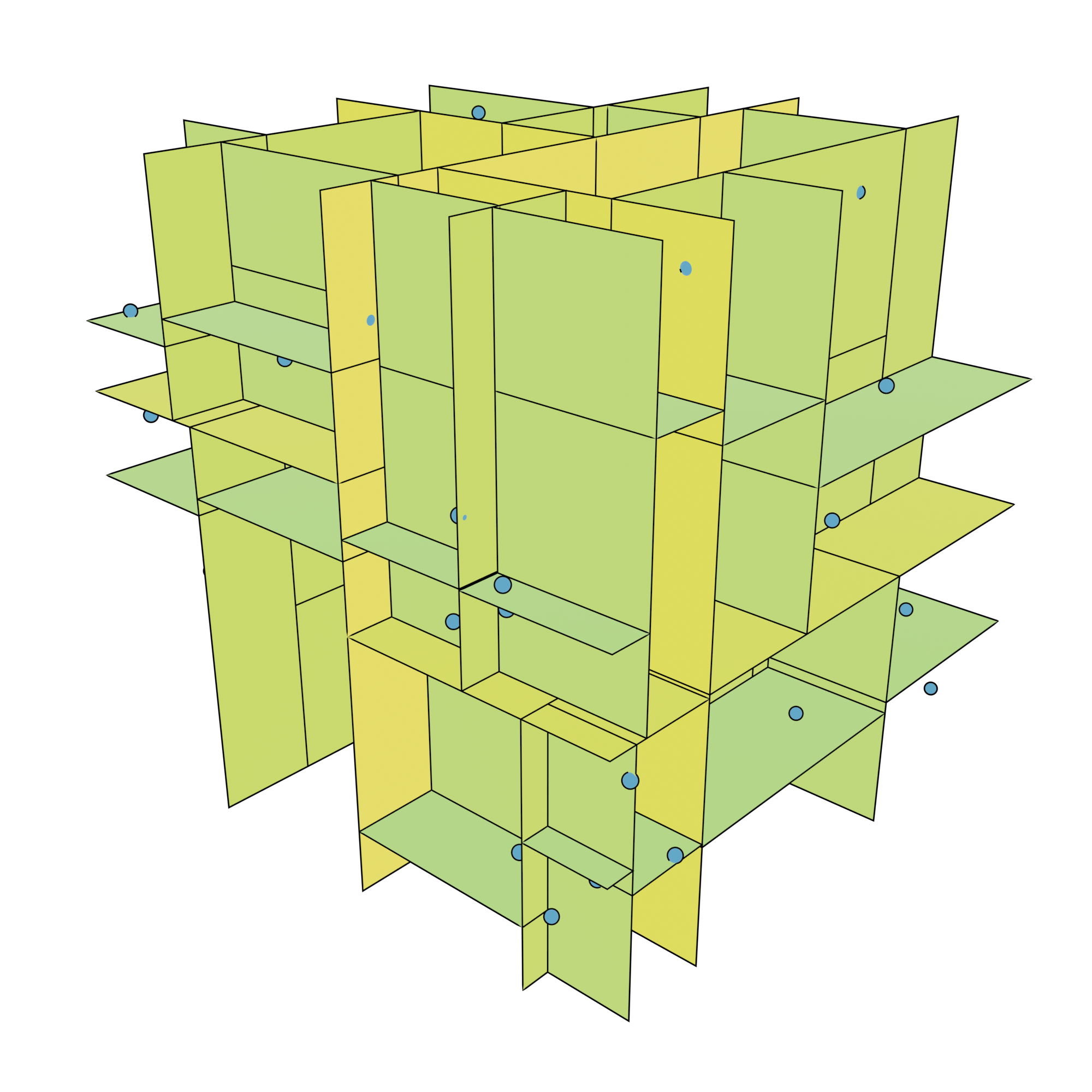
The canonical approach to computing nearest-neighbors is a -d tree - a class of space partitioning tree. There are many formulations, but I'll use a median-partitioning tree in this case.
At each branch of a -d tree, we split the the space into two sub-volumes, each containing the same number of points, based on the median value along one dimension. For instance, if we wanted to split the points along the first dimension, we'd choose a split value of 3, and if we were splitting along the second dimension, we'd choose a split of 3.5. For efficiency, we'll have our tree split first on dimension 0 (), then dimension 1 (), and so on, until looping back around to dimension 0.
When querying the nearest neighbor, we first do a quick binary search of the tree to find a candidate closest point. Next, we perform a branch-and-bound search of every other subtree, escaping early if the test point is further from a volume from the candidate-closest point. I'm staying light on the exact details here, since the point of this article is not to explain how -d trees work.
These are very nice data structures, but they suffer from two core issues for our application: first, -d trees have extremely poor cache locality due to the fact that they jump around everywhere during a search. Second, this approach is not at all amenable to SIMD parallelism, which typically requires some amount of branchlessness. How do we make something which is similarly performant (or better!) without the same limitations?
Being stupid faster
We can start by noticing a neat quirk of the first pass on a -d tree: the first downward pass can be done completely branchlessly and in a very cache-friendly way. To do so, we'll need to bring out a special data layout for trees, called an Eytzinger layout. This Algorithmica article gives a beautiful explanation of it, but I'll try my own hand at an explanation as well.

In an Eytzinger layout, we implicitly describe the location of each branch in the tree by its location in a
buffer. We store all the tests in some array (let's call it
tests for convenience), and for some branch-point at index , the left child will be at position
, while the right child will be at position
. If we assume that the number of points in the tree is a power of 2, and that the tree is perfectly balanced,
we can create an extremely efficient method for the first pass through the tree. If the number of points is not
a power of two, we can just pad the point cloud with points at .
struct ForwardTree {
    /// contains 2^p - 1 tests
    tests: Box<[f32]>,
    /// contains 2^p points
    points: Box<[[f32; 3]]>,
}

/// Return the index representing
/// the cell in the tree containing `point`.
fn first_pass(tests: &[f32], point: &[f32; 3]) -> usize {
    let mut k = 0;
    let mut i = 0;
    while i < tests.len() {
        i = 2 * i + 1 + usize::from(tests[i] < point[k]);
        k = (k + 1) % 3;
    }

    i - tests.len()
}
This first pass computes a usize identifying which point in points is closest to
point. Approximation isn't really good enough for collision checking, but we'll find some other
tricks for that later. For now, we'll notice that it's pretty easy to render this code as a parallel
implementation using the nightly portable_simd feature for Rust.
use std::simd::{prelude::*, LaneCount, Simd, SupportedLaneCount};

fn first_pass_simd<const L: usize>(
    tests: &[f32],
    points: &[Simd<f32, L>; 3],
) -> Simd<usize, L>
where
    LaneCount<L>: SupportedLaneCount,
{
    let mut k = 0;
    let mut i = Simd::splat(0);
    let nlog2 = tests.len().trailing_ones();
    for _ in 0..nlog2 {
        let tests = Simd::gather_or_default(tests, i);
        let cmp = points[k].simd_ge(tests).to_int().cast();
        let one = Simd::splat(1);
        i = (i << one) + one + (cmp & one);
        k = (k + 1) % 3;
    }

    i - Simd::splat(tests.len())
}
The above code does the exact same thing as first_pass, but this time in parallel across a set of
L different robot spheres. This means we can get a speedup of up to L times on
whole-robot collision checks.
Once we've extracted the identifier for our approximate-nearest-neighbor, we can do a quick test for whether it's in collision by computing the distance to the center of the query sphere.
/// If this returns `true`, a sphere centered at `point`
/// with radius-squared `rsq` collides with a point in `t`.
/// May erroneously return `false`.
fn forward_coll(t: &ForwardTree, point: &[f32; 3], rsq: f32) -> bool {
    let id = first_pass(&t.tests, point);
    point
        .iter()
        .zip(t.points[id])
        .map(|(&x, y)| (x - y).powi(2))
        .sum::<f32>()
        <= rsq
}
Of course, we can also do our collision checking in a SIMD parallel manner; however, the resulting code would be rather verbose and not very interesting. Since we'll need to throw that code away shortly anyway, I'll skip ahead to the good part, which is the performance results.
At these scales, a
-d tree is the best competitor. Fortunately, kiddo, one of the fastest -d tree implementations out there, is easy to install via Cargo. I'll be using that as a rough baseline for
point cloud collision-checking. I found that the fastest results came from using within_unsorted on
an ImmutableKdTree, so I'm using that as my baseline.

We see that this single-pass approach blows a normal
-d tree out of the water, yielding enormous speedups in query time from hundreds of nanoseconds to only about
10 ns. Sadly, the SIMD addition is only a modest improvement - this is because gather instructions are very slow
on my laptop's processor. On other machines, there's usually a more appreciable performance improvement. This
comparison also isn't really fair: kiddo is giving us an exact answer to whether we're in
collision, while our forward tree is only returning an approximate answer.
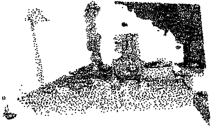
Not only that, our approximate answer isn't even all that good. To test this, I collected a real point cloud and measured the distribution of position error when selecting nearest neighbors.

Looking from the cumulative distribution function above, we see that roughly 20% of points have an error of over 10 cm. In the world of collision checking, that's enormous - any padding conservative enough to make this forward tree useful would make it impossible for a robot to find a plan.
Missing the forest for the trees
My first idea for fixing this error issue was very simple: if one tree was only right some of the time, we could get the results from multiple trees and (hopefully) improve our accuracy.
This is not a new idea, per se: random forests are pretty well known in the ML community. The core concept is this: we make different trees. Each tree is randomly different somehow, yielding typically incorrect errors. We can then take the best result from each tree for a (hopefully) dramatic improvement in result quality.
struct RandomTree {
    tests: Box<[f32]>,
    points: Box<[[f32; 3]]>,
    seed: u32,
}
For the sake of branchless parallelism, we'll randomize each tree according to a pseudo-random number generator. Then, when we search through the tree, we determine the next axis to branch on based on the outcome from the RNG.
/// A simple PRNG.
fn xorshift32(x: &mut u32) -> u32 {
    *x ^= *x << 13;
    *x ^= *x >> 17;
    *x ^= *x << 5;
    *x
}

fn first_pass_rand(tests: &[f32], mut x: u32, point: &[f32; 3]) -> usize {
    let mut i = 0;
    while i < tests.len() {
        let k = xorshift32(&mut x) as usize % 3;
        i = 2 * i + 1 + usize::from(tests[i] < point[k]);
    }

    i - tests.len()
}
An astute reader might note that this implementation branches on the same dimension for each depth in each random tree, independent of which subtree we search. This is intentional: it makes it easier to write a branchless SIMD implementation of random tree querying. Otherwise, we'd need a convoluted sequence of shuffles to get every element in the correct lane, which would chew up the performance.
Young and full of hope, I tried checking the error distribution of the random forest approach. I constructed a point cloud, randomly generated a bunch of query points, and tested those points for their distance to their nearest neighbor in the cloud.

When testing the error distribution for a forest, the results are less than impressive. We get diminishing returns at around 4 trees in the forest, with minimal gains from adding trees past that. Even with 10 trees in the forest, our maximum error could be as much as 20 cm.

Even if that error distribution were better, queries to these forests exhibit superlinear scaling with the number of trees, since together they use so much memory that they can't all fit in the cache. At around 10 trees, the SIMD performance of a forest is about the same as a -d tree, but as we discussed before, the error isn't good enough to justify using it.
A budget for affording
Let's briefly take stock of the situation. Using our forward tree, we can quickly classify a query point as belonging to a single unit cell. We know that for any fixed cell and radius of a test-sphere, there is a fixed set of points in which are close enough to collide with at least one point in the cell. If we're targeting a particular robot, we also know , the maximum radius of a sphere on the robot. If we trust that we'll never do a collision check for a sphere larger than , then any query point in a given cell can only ever collide with a fixed set of points in the cloud: namely, the set of points whose distance to the cell is less than or equal to .

Let's call those points afforded; that is, for a given cell and a radius , affords if there exists a point such that .
Using our knowledge of , we can annotate each leaf of our forward-tree with the list of all afforded points. Then, when checking for collision, we can traverse this list of afforded points and test for collision against any of them. This allows us to convert our approximate-nearest-neighbor guess into a completely accurate range-nearest-neighbors query without . I currently call the resulting structure an collision-affording point tree, or CAPT for short.
Now, instead of storing a single point for each leaf of the tree, we'll store a list of points which might be in collision, called an affordance set.
struct Capt {
    tests: Box<[f32]>,
    afforded: Box<[Box<[[f32; 3]]>]>,
}
However, this data layout isn't quite optimal. We've broken up our possibly-colliding points into a bunch of different allocations, requiring an extra size parameter on each and fragmenting our memory. We can coagulate all the affordance set into one gigantic array, and then use another lookup table to get the starting and ending indices relevant to one point.
Additionally, to make SIMD parallelism easier, we can use a struct-of-arrays layout for each point in
afforded, which means that we split out each dimension of every point, and store them in separate
buffers.
struct Capt {
    /// contains n - 1 elements
    tests: Box<[f32]>,
    /// contains n + 1 elements
    starts: Box<[usize]>,
    /// each buffer contains aff_starts[n] elements
    afforded: [Box<[f32]>; 3],
}id from first_pass,
afforded[starts[id]..starts[id + 1]] will contain all the afforded points for the cell.
fn capt_collides(t: &Capt, point: &[f32; 3], rsq: f32) -> bool {
    let id = first_pass(&t.tests, point);
    (t.starts[id]..t.starts[id + 1]).any(|i| {
        t.afforded
            .iter()
            .zip(point)
            .map(|(a, &b)| (a[i] - b).powi(2))
            .sum::<f32>()
            <= rsq
    })
}
If we tried to parallelize collision-checking between our query spheres and afforded points like we did in
first_pass, we wouldn't actually see much performance benefit. I know this because that's what I
had originally tried, and it was hardly faster than the sequential implementation. The heart of the problem is
that gather instructions are comically slow on nearly all processors, so the CPU spends far more time waiting
for memory to arrive than it does on churning through computations.
To fix this, we need to have a way to test for collision without touching a large about of memory at the same
time. The simplest fix is the best: instead of parallelizing across queries, we parallelize across afforded
points for one query. We iterate sequentially through the query spheres, but in parallel, we check whether
L different afforded points collide with the same sphere. The upside of this is that the data for
these points are stored contiguously, so we waste no time waiting on gathers.
fn capt_collides_simd<const L: usize>(
    t: &Capt,
    points: &[Simd<f32, L>; 3],
    radii: Simd<f32, L>,
) -> bool
where
    LaneCount<L>: SupportedLaneCount,
{
    let ids = first_pass_simd(&t.tests, points);

    let start = Simd::gather_or_default(&t.starts, ids);
    let end = Simd::gather_or_default(&t.starts, ids + Simd::splat(1));

    for l in 0..L {
        let pt = [0, 1, 2].map(|k| Simd::splat(points[k][l]));
        let rsq = Simd::splat(radii[l].powi(2));
        for s in (start[l]..end[l]).step_by(L) {
            let mut distsq = Simd::splat(0.0);
            for (pt_k, aff_k) in pt.iter().zip(&t.afforded) {
                // assume `affordances[k]` is sufficiently long
                // for simplicity
                let diff = pt_k - Simd::from_slice(&aff_k[s..]);
                distsq += diff * diff;
            }
            if distsq.simd_le(rsq).any() {
                return true;
            }
        }
    }

    false
}
Squeezing out some juice
The performance of this "default" tree is pretty good, but there's one place where it suffers a lot: non-colliding queries. If a query sphere doesn't collide with any afforded point, we have to check every single afforded point. Some cells could afford hundreds of points, which would yield extremely poor runtimes. We need some sort of fast-path rejection for queries which are certainly not in collision.
Getting in order
I first observed that many query spheres had much smaller radii than the maximum afforded radius of the tree. This means that many of the afforded points for each cell would be further from the cell than the query radius, meaning that they could never collide with a query sphere of that radius.

The first idea we had for this was to sort all the points in each affordance set in descending order of distance to the cell. That way, searches with small query radii would be able to terminate earlier: as soon as the collision-check found a point further from the cell than the query radius, the search could terminate immediately.
This was good for query performance, but came at a significant cost in tree construction time. I'll explain the details of construction later in this post, but for now, know that this measure put construction times into the worst-case regime of for trees containing points. This is far too much time when is measured in thousands; in some of my tests it took 30 seconds to construct the tree on large point clouds. In the end, I had to nix this feature for performance.
Shrinking down

While experimenting, I found that a very small minority of cells had extremely large affordance sets. These cells were typically very small, and in the middle of a big cluster of points. Often, because the cells were so small, every single query sphere inside the cell would collide with the representative point of the cell.
I decided to take advantage of this to reduce the peak affordance size. We already accept that we know , so why not also provide a minimum radius ? If a sphere of radius collides with a point, then any other query sphere with the same center should also collide, no matter what. For the small cells, then, we can throw away all other points except the representative point of the cell and store only a single point in its afforded set.
Bounding my boxes

There's one last notable case where the search spends a lot of time needlessly checking for collisions. Cells near the edge of a cluster are often long and skinny, with one tip of the cell being very close to the cluster and the other tip extending far out into space. Those long, skinny cells often take up the majority of the free space in the environment, meaning most of our queries will actually be against a cell which is mostly empty.
We'd like to be able to filter out queries which aren't in collision as fast as possible, ideally skipping the lengthy affordance set check. Since often only one part of the cell contains afforded points, this opens up a possibility for improvement: what if we just didn't check the spheres in the "empty" part of the cell?
To do this, we construct an axis-aligned bounding box (AABB) containing the affordance set for each cell. If we're lucky, the AABB will often be much smaller than its cell.
struct Capt {
    /// contains n - 1 elements
    tests: Box<[f32]>,
    /// contains n elements
    aabbs: Box<[Aabb]>,
    /// contains n + 1 elements
    starts: Box<[usize]>,
    /// each buffer contains aff_starts[n] elements
    afforded: [Box<[f32]>; 3],
}

#[derive(Clone, Copy)]
struct Aabb {
    lo: [f32; 3],
    hi: [f32; 3],
}
Then, when querying, we can cheaply detect whether a query sphere intersects the AABB. If it doesn't, then we know that the sphere is not in collision, and can avoid later expensive steps in collision-checking.
fn intersects(aabb: &Aabb, center: &[f32; 3], rsq: f32) -> bool {
    aabb.lo
        .into_iter()
        .zip(aabb.hi)
        .zip(center)
        .map(|((l, h), x)| |((l, h), x)| (x.clamp(l, h) - x).powi(2))
        .sum::<f32>()
        <= rsq
}

/// Rewritten from the previous version.
fn capt_collides(t: &Capt, point: &[f32; 3], rsq: f32) -> bool {
  let id = first_pass(&t.tests, point);
  intersects(&t.aabbs[id], point, rsq)
      && (t.starts[id]..t.starts[id + 1]).any(|i| {
          t.afforded
              .iter()
              .zip(point)
              .map(|(a, &b)| (a[i] - b).powi(2))
              .sum::<f32>()
              <= rsq
      })
}
With that, we have the complete collision-checking logic for a CAPT. The process is simple: classify a query sphere as belonging to a cell, then check whether the query sphere collides with any points sufficiently close to the cell. This step can also be parallelized using SIMD by batching collision checks with a set of afforded points in a cell; however, I'm not including the sample code for that since it's quite complicated.

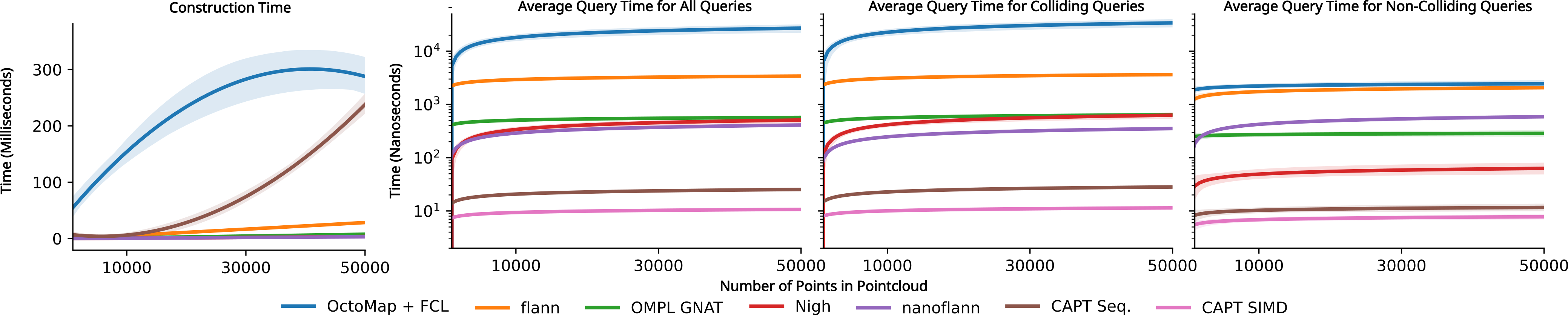
To see how well this tree performs, I'm showing the results from a benchmark above. This plot shows the relative throughput of various methods on a sequence of collision-checking queries. These queries were recorded from a real motion planning problem, then I played the same sequence of queries back with just the collision-checking to see how much each collision-checking procedure took. All the numbers for the Rust implementation were recorded on my laptop, though our paper's benchmarks ran on a somewhat beefier desktop computer.
We see that the CAPT is only slightly slower than the naive forward-only tree. For some reason, it slows down dramatically once there are enough points: this only occurs on my laptop, so I suspect it has something to do with cache locality weirdness.
Under construction


After all this, I still haven't explained how these trees are constructed. Efficiently constructing a CAPT is nontrivial, since the brute-force approach to affordance set construction is a total non-starter. Luckily, the construction procedure is much like that of a normal -d tree.
We start out given some list of points , our point cloud. Since our Eytzinger-layout-based search procedure requires to be a power of two, we compute , which is the next power of two after , and then pad to length with points at to produce .
Next, we recursively partition the tree, maintaining a candidate affordance set , initialized as an empty set; and a candidate volume , initialized to the axis-aligned bounding box containing all of . We partition by the following steps:
- Compute the median plane for the current cell.
- Split the cell by the median plane into two smaller cells, and . Split the points in the cell into two subsets: those below the median plane and those above the median plane; call them and .
- Construct new affordance sets and , such that and .
- Filter out all points in which are not afforded by at radius . Do the same for and .
- Recursively repeat this process for both partitioned cells until each cell contains only one point.
I'm intentionally avoiding code in my description here because the code required to construct the tree is quite verbose. I've made a stripped-down version in the spoiler block below for completeness, though.
*deep breath*
First, a helper function for determining whether a sphere contains all of a cell:
fn sphere_contains(center: &[f32; 3], rsq: f32, vol: &Aabb) -> bool {
    vol.lo
        .into_iter()
        .zip(vol.hi)
        .zip(center)
        .map(|((l, h), c)| if c - l < h - c { h - c } else { c - l }.powi(2))
        .sum::<f32>()
        <= rsq
}
We start by padding the points to a power of two, then immediately call out to a helper function to populate all the buffers.
fn capt_new(points: &[[f32; 3]], r_range: (f32, f32)) -> Capt {
    let n2 = points.len().next_power_of_two();
    let mut points2: Vec<_> = vec![[f32::INFINITY; 3]; n2];
    points2[..points.len()].copy_from_slice(points);
    let mut tests = vec![f32::NAN; n2 - 1].into_boxed_slice();
    let mut afforded = [Vec::new(), Vec::new(), Vec::new()];
    let mut starts = vec![0];
    let mut aabbs = Vec::new();

    capt_new_help(
        &mut points2,
        &mut tests,
        &mut aabbs,
        &mut afforded,
        &mut starts,
        0,
        0,
        r_range,
        Vec::new(),
        Aabb {
            lo: [f32::NEG_INFINITY; 3],
            hi: [f32::INFINITY; 3],
        },
    );

    Capt {
        tests,
        aabbs: aabbs.into_boxed_slice(),
        starts: starts.into_boxed_slice(),
        afforded: afforded.map(Vec::into_boxed_slice),
    }
}
Next, we write the main recursive helper function for splitting up cells and populating the affordance sets. If this looks convoluted, remember that the version used in the final code was even worse.
#[allow(clippy::too_many_arguments)]
fn capt_new_help(
    points: &mut [[f32; 3]],
    tests: &mut [f32],
    aabbs: &mut Vec<Aabb>,
    afforded: &mut [Vec<f32>; 3],
    starts: &mut Vec<usize>,
    k: usize,
    i: usize,
    r_range: (f32, f32),
    in_range: Vec<[f32; 3]>,
    cell: Aabb,
) {
    // Base case: only one point in the cell means this is a leaf
    if let [rep] = *points {
        // AABB of all afforded points
        let mut aabb = Aabb { lo: rep, hi: rep };

        // Exclude padded infinites from affordance sets
        if rep[0].is_finite() {
            // Representative point comes first
            (0..3).for_each(|k| afforded[k].push(rep[k]));
            // Don't include other points if the cell is small enough
            if !sphere_contains(&rep, r_range.0.powi(2), &cell) {
                for p in in_range {
                    for k in 0..3 {
                        // Expand AABB to contain afforded points
                        if p[k] < aabb.lo[k] {
                            aabb.lo[k] = p[k];
                        } else if aabb.hi[k] < p[k] {
                            aabb.hi[k] = p[k];
                        }
                        afforded[k].push(p[k]);
                    }
                }
            }
        }
        // Update starts to match this region of afforded
        starts.push(afforded[0].len());
        aabbs.push(aabb);
        return;
    }

    // Recursive case: splitting a cell

    // Compute the median plane of the cell
    let (lh, med_hi, _) = points
        .select_nth_unstable_by(points.len() / 2, |a, b| {
            a[k].partial_cmp(&b[k]).unwrap()
        });
    let med_lo = lh
        .iter()
        .max_by(|a, b| a[k].partial_cmp(&b[k]).unwrap())
        .unwrap();
    let test = (med_lo[k] + med_hi[k]) / 2.0;
    tests[i] = test;

    // Split the volumes
    let mut lo_range = in_range.clone();
    let mut hi_range = in_range;

    let mut lo_vol = cell;
    lo_vol.hi[k] = test;
    let mut hi_vol = cell;
    hi_vol.lo[k] = test;

    // Compute the new afforded sets
    lo_range.retain(|p| intersects(&lo_vol, p, r_range.1.powi(2)));
    hi_range.retain(|p| intersects(&hi_vol, p, r_range.1.powi(2)));

    let (lhs, rhs) = points.split_at_mut(points.len() / 2);
    lo_range.extend(rhs.iter().filter(|p| p[k] <= test + r_range.1));
    hi_range.extend(lhs.iter().filter(|p| p[k] >= test - r_range.1));

    // Recur for each half of the split
    capt_new_help(
        lhs,
        tests,
        aabbs,
        afforded,
        starts,
        (k + 1) % 3,
        2 * i + 1,
        r_range,
        lo_range,
        lo_vol,
    );

    capt_new_help(
        rhs,
        tests,
        aabbs,
        afforded,
        starts,
        (k + 1) % 3,
        2 * i + 2,
        r_range,
        hi_range,
        hi_vol,
    );
}
Unfortunately, even with some extra engineering work, our construction times for the tree still sucked. I even tried transforming the recursive construction procedure into a stack-based iterative one. At the end of the day, the core problem is simply algorithmic: if the average affordance-set size is , and there are points, construction takes roughly time for sufficiently large . In most cases, grows with , so it could perform as slowly as in some clouds. For a cloud with a few hundred thousand points, that's completely untenable.
Filter feeders
The most natural solution to our construction time problem is to reduce the size of our point clouds. There are many ways to do this, and the simplest way is to just uniformly randomly sample points from the cloud until we have the desired quantity. However, most methods provide few guarantees about the quality of the sampled cloud. Ideally, we want to downsample the cloud to reduce its density as much as possible; however, we can't downsample so much that we hallucinate a gap in the cloud and produce an invalid plan. Accordingly, we'll need a more intelligent filtering scheme.
While we were thinking about filtering point clouds, we were also thinking about efficient construction algorithms for the tree. One idea we had played with was implicit representation for afforded sets. The hope was that we could store less data while constructing the tree and filter out affordance sets in time. One such approach used segments of a space-filling curve to represent sets of points, which would hopefully have allowed us to slice up affordance sets much more efficiently.
Unfortunately for us, that approach never worked out, and so we were stuck with our bad construction times. However, we still had the idea of space-filling curves on our mind when we were thinking about filtering the point cloud. How could we use a space filling curve to filter out point clouds more efficiently?
I'll start with a simple example. Suppose we have a list of points in one-dimensional space; that is, a list of real numbers, and we want to filter it to reduce its density, but still preserve the areas where points are in collision. In particular, we might want to make sure that if some point is removed, there exists another point which was not removed, such that is less than some radius . In that case, filtering our list of points would be easy: we sort the points in order, then remove one of every adjacent pair if .
With a bit of cleverness, we can generalize this approach to arbitrarily many dimensions. The trick is to instead sort the points along a space-filling curve, which will place nearby points approximately near each other when sorted.

The best-known space-filling curve is the Hilbert curve, but it's relatively convoluted to compute. Instead, we used a Morton curve (also known as a Z-order curve), because it's trivial to compute a point's position along a Morton curve using a parallel-bits deposit instruction.
use bitintr::Pdep;
use std::ops::BitOr;

/// Compute `p`'s position along the Morton curve filling `aabb`.
fn morton_index(p: &[f32; 3], aabb: &Aabb) -> u32 {
    const MASK: u32 = 0b001_001_001_001_001_001_001_001_001_001;

    // the magic 1024 comes from the fact that MASK has 10 bits set,
    // so we scale up the position of `p` along each axis to have 10 bits
    // per dimension.
    p.iter()
        .enumerate()
        .map(|(k, x)| {
            (((x - aabb.lo[k]) * 1024.0 / (aabb.hi[k] - aabb.lo[k])) as u32)
                .pdep(MASK << k)
        })
        .fold(0, BitOr::bitor)
}
The main downside to using the space-filling curve filter is that there are "cliffs" - regions where moving a small amount in space dramatically changes your position on the space-filling curve. To fix this, we can just filter the point cloud multiple times. Each time, we'll use a different Morton curve (one for each permutation of dimensions) in the hopes that using different filters will give us more opportunities to filter points.

In practice, this yields some pretty great results! One filter pass can dramatically reduce the size of a point cloud, even at a small radius. In the plot above, I've run up to 6 different filters over a point cloud of a bookshelf containing points. Looking at the plot above, we get some diminishing returns from filtering with more permutations. However, since the construction performance is so superlinear, it's still worthwhile to do some extra filtering in the hopes of reducing point cloud size a little further.
We also played around a little bit with scaling dimensions of the Morton filter. We started by stretching and transforming the space such that the region gets mapped to the AABB containing all the points in the point cloud. Since the filter removes some points on the edge of that AABB, we tried shrinking the AABB to fit the new sparsified point cloud for the next iteration of the filter, and we also tried leaving it as-is. For reasons I can neither explain nor comprehend, the most effective way was to take an average of the two AABBs to produce the best filtering results.
Into the C++ mines
I hate C++. This isn't a place for unhinged ranting about programming languages, but let it be known that I do not write C++ willingly or lightly. However, the vector-accelerated motion planner that I was developing for was written in C++, and there's no shot of it getting rewritten in the near future. We all have better things to do. Instead, I got to reimplement all the Rust prototype code in C++.
On the whole, it wasn't as bad as it could have been, but a small part of me dies inside every time I have to read a template instantiation error message. My Rust implementation (not the simplified version in this blog post) was polymorphic over dimension, but I only had to implement the C++ version for , which made things easier.
We spent a little more engineering effort on construction and query times for the C++ code, in part by taking advantage of some domain-specific knowledge. This let us eke out a little more performance, so the Rust code is marginally slower, but not due to any differences in programming languages.
I spent a lot of time debugging quirky results. For reasons I still have yet to understand, the SIMD queries performed worse on SIMD-parallel queries than they did on sequential queries. However, this result exclusively ocurred on the C++ implementation on my laptop - no other machines. The solution? Simply run the benchmarks on a different machine.
The final scramble
What I've described so far was roughly the state of the project around two weeks before the submission deadline. However, it takes more than a good idea to produce a good paper. We needed serious benchmarks against serious competitors. Since the state of C++ software packaging is practically nonexistent, this typically entailed vendoring the source code as a Git submodule, patching it into the CMake build system, and praying that it would compile. Repeat for each competitor and we've got a full set of benchmarks.
We really cared about a few main competitors: OctoMaps and -d trees (in the C++ implementation nanoflann and Nigh). OctoMaps are a big deal in the planning world, and tend to be the most common off-the-shelf environment representation for point clouds, while comparing against -d trees would prove that our SIMD and cache-efficiency efforts actually did something. We benchmarked against a handful of others, but this blog post is far too long for me to go into detail about all of them.
| Collision-Checker | Filter | Build | Plan | Simplification | Total |
|---|---|---|---|---|---|
| OctoMap | 2.9 | 120.9 | 78.9 | 23.3 | 220.9 |
| nanoflann | 0.3 | 15.5 | 7.8 | 26.7 | |
| CAPT | 5.9 | 0.5 | 0.2 | 9.5 |
When hooked up to a full motion planner, we found that we could get speedups by multiple orders of magnitude. Planning times fell from the order of tens to hundreds of milliseconds using an OctoMap down to microseconds with our data structure. From end to end, we could go from a raw point cloud all the way to a completed plan in under sixteen milliseconds. That means that sixty-hertz online planning times are possible!
For the final benchmarks, instead of using my laptop, we used a much beefier computer with a Ryzen 9 7950X, which accounts for the biggest difference in empirical performance compared to the earlier plots. We were actually quite surprised by our results - we weren't expecting to be that far ahead.
Our target conference was Robotics: Science and Systems, which is a relatively small yet competitive venue. Typically, they have high standards for submission quality, so we were worried about about making the cut, especially on a tight deadline. We ended up divvying up the work for the paper: I was mostly responsible for writing up the method, related work, some analysis, and results, while my collaborators Wil and Zak wrote up the intro and added their own parts to the stuff that I had drafted. Lastly, my advisor, Lydia, reviewed and edited the paper.
We wanted to benchmark against nvblox, but it was a nightmare to get it to compile and run on anything. I managed to obliterate my graphics drivers twice while setting up the requisite CUDA drivers, and had to reinstall the OS from scratch. In the end, we just gave up.
Software hell
We also tried to get the planning system running on a real robot. The first hurdle was exfiltrating a point cloud from the RealSense camera, which proved surprisingly difficult, mostly because I believe that software was invented as some sort of cruel punishment for my sins. We only managed to get the imaging stack working late around 3 A.M. on the night the paper was due. In my experience, my productivity drops off dramatically around 10 P.M., so perhaps that was only two hours of "real" work, but it was still far more difficult than getting a list of points in the correct coordinate frame should be. Armed with our point cloud, we were able to get real-enough demo results for the paper.
Victory laps
Like many other venues, RSS has two different submission deadlines: the paper deadline and then the supplemental materials submission a week later. This meant that we had enough time to try to get an online planner running, hopefully to demonstrate camera-frequency planning. However, we ran up against a new problem: we were planning too fast.
The heart of the issue was ROS's trajectory blender: by and large, it assumes new trajectories are provided only once every few seconds. However, our planner could produce hundreds of plans per second with ease: at that frequency, the trajectory blender could not keep up and so it yielded inconsistent, jerky motions.
We didn't have time to fully fix the issue before the submission deadline, but a few days later we managed to finally get things running. Our solution was to instead manually implement a velocity controller for the robot and dodge the ROS interface entirely.
Eventually, we got the whole thing running! In the demo video above, the robot attempts to move to a sequence of preset positions. At every single camera frame, we scan a point cloud, build an environment, and then compute an entirely new plan from scratch - roughly sixty times per second. This means that we can insert arbitrary obstacles in the scene and it all "just works": the robot magically dodges them all.
We had to do a few hacks to get this to all work, though. The big issues weren't actually from our planner performance but rather from perception: occlusion from solids meant that we could only perceive the surface of obstacles, so we had to pad the radii of all points by 4cm just to make it so that the robot wouldn't crash into the underside of the pool noodles. Additionally, if we ever stuck a pool noodle under the robot, the robot would occlude those points and then happily drive itself through it.
Reviewer 2 is real
About a month after we submitted the paper, we got reviews back. Most of the remarks were things we already knew, but there was one major hiccup - our proof of correctness. From our filtering method, we knew that if any point was removed from a point cloud, we would leave a point such that . From that, we derived a proof that this filter wouldn't produce gaps (based on the dispersion of the point cloud), and from there on we proved that the whole pipeline was correct. However, we didn't explain which definition of dispersion we were using, and so there were maybe ten people on the planet who would have had a chance at understanding what we claimed at all.
The reviewers rightfully called us out on such nonsense, and thankfully, there is a definition of dispersion which does make this proof work (see LaValle, Planning Algorithms, sec. 5.2.3), so we got away with it in the end.
Becoming a marketer
I think you shoulg go to Japan
Very little of an academic's time is spent doing worthy research; instead, they mostly try to convince others that their research is worth doing. For the entirety of April and May, my efforts have been mostly directed that way: preparing materials and advertising my work.

I started out small with a poster presentation at TEROS, a small symposium at Texas A&M. When I printed the poster, however, I picked the wrong version: I printed a PDF with feedback attached as comments. I only found out that my poster was covered in yellow highlights when I arrived. It was too late to fix, so I just didn't mention the highlighting to anyone else. In spite of this, I had a pretty fun time there, and it seems like there were a handful of people interested in the work.
At my university, first-year Ph.D. students are given a $2500 grant for either conference travel or a laptop to be spent in their first year. By March, I hadn't spent any of that grant money, since my current laptop was still working correctly. Accordingly, I got the above email header from my advisor, Lydia - ICRA 2024 was in Yokohama, Japan this year, and I showed up at a workshop with a trimmed-down version of my paper.

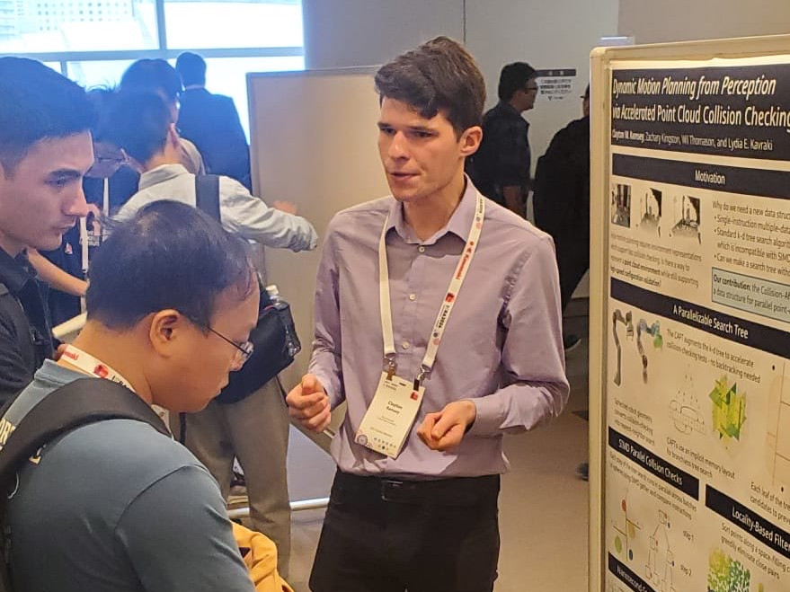
ICRA was my first conference, and I thought it was pretty cool! I got to see a lot of really exciting work from across the field, and it seems like a number of people were also excited about my work. To be completely honest, I also found that the oral presentations were simply not worth it - it's too easy to zone out, and it's never at the right amount of detail. Instead, the best place to hang out is in the poster presentation area, because you can talk directly to the authors and get a much better sense of their work.
The last major bit of marketing was of course this blog post; though, to be honest, it's more for my personal pleasure than it is to try to drum up interest.
Terminus
The last few months of my degree has been a lot of work, but also a lot of fun! I originally hadn't believed that I could get all this done in such a short time. I'll admit, I've sort of impostor-syndromed myself: my advisor, Lydia, was very impressed with my work, but it feels to me that my collaborators, Wil and Zak, did a lot of the "real" work. Now expectations are higher, and I have to figure out how to make something this good again.
That being said, I'm still pretty excited for the future! I think this is a good first step for my research, and it's opened up a lot of avenues for me. There are a lot of applications for fast planning out there, and I'm thinking that I can explore a few to get a full thesis.